[1] "Long continuous observations: 7034"[1] "Long categorical observations: 4577"Provide a detailed descriptive analysis of the dataset, including marker distributions, molecular subtypes, and comparisons between Pre-AI and Post-AI assessments.
Note for Pathologist: This report summarizes the overall characteristics of the cases included in the study. We look at the distribution of biomarker values (ER, PR, Ki67, HER2) and molecular subtypes before and after AI assistance. This helps us understand the “baseline” of our data and how AI might be shifting the overall distributions. All analyses here are based on the set of cases evaluated by all pathologists.
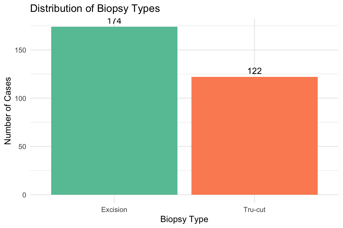
[1] "Long continuous observations: 7034"[1] "Long categorical observations: 4577"[1] "Number of Cases: 296"[1] "Number of Pathologists: 4"[1] "Total Assessments: 1184"Distribution of cases by biopsy type (Excision, Tru-cut). Vacuum-assisted biopsies were recoded as Tru-cut.
| Distribution of Biopsy Types | ||
| Biopsy Type | Number of Cases | Percentage (%) |
|---|---|---|
| Excision | 174 | 58.8 |
| Tru-cut | 122 | 41.2 |
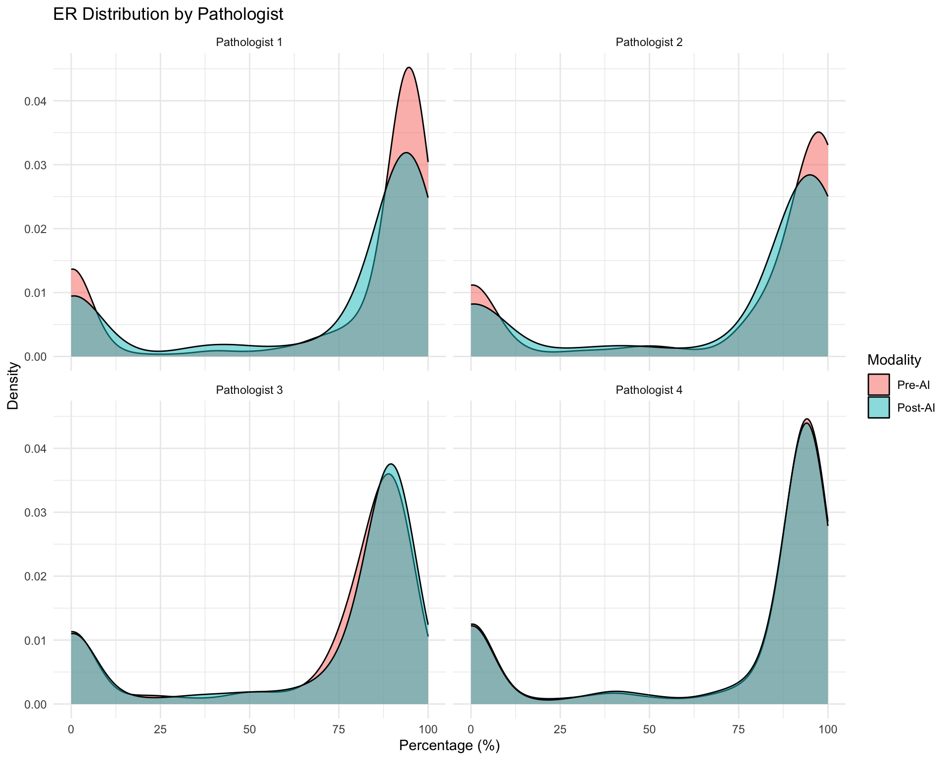
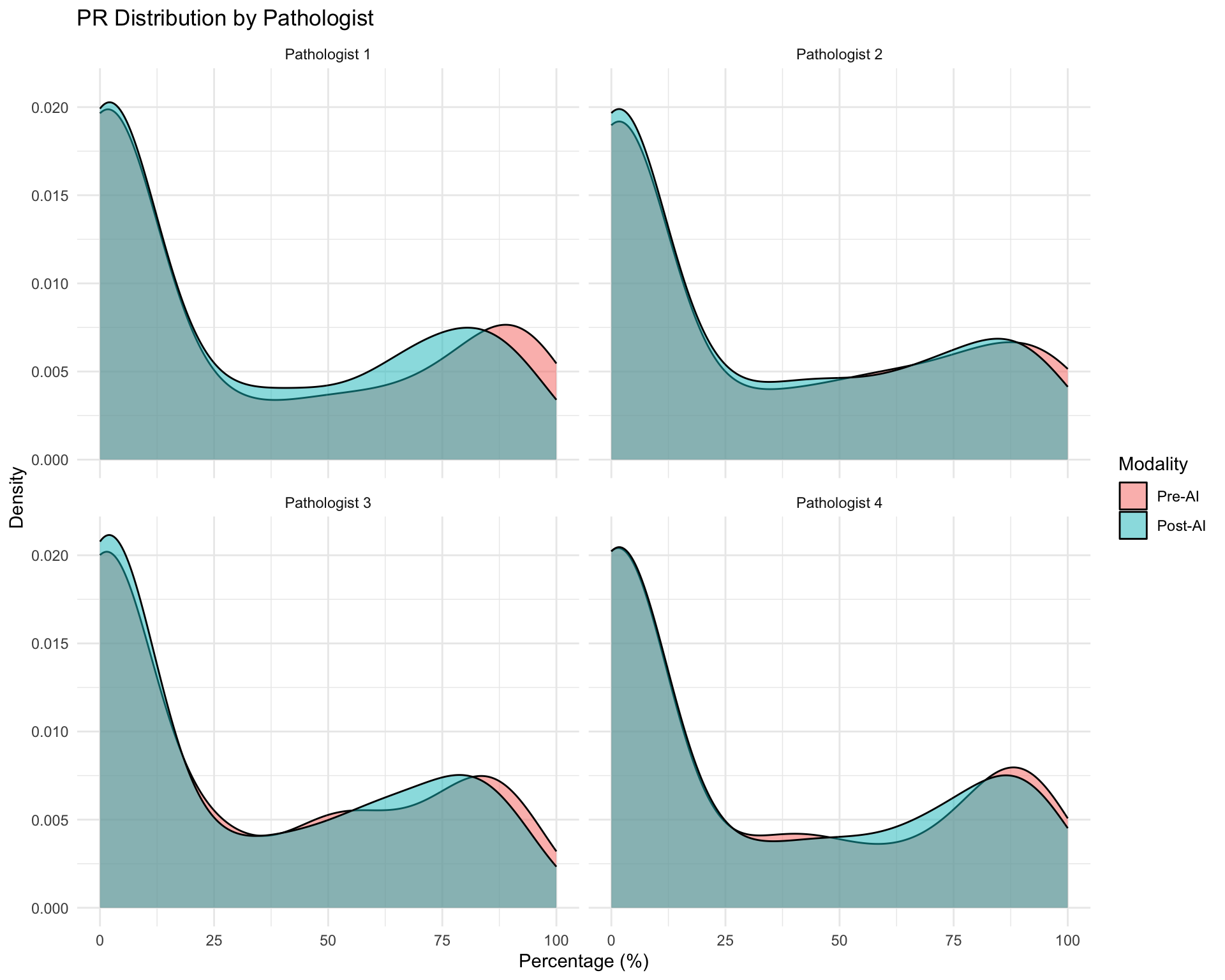
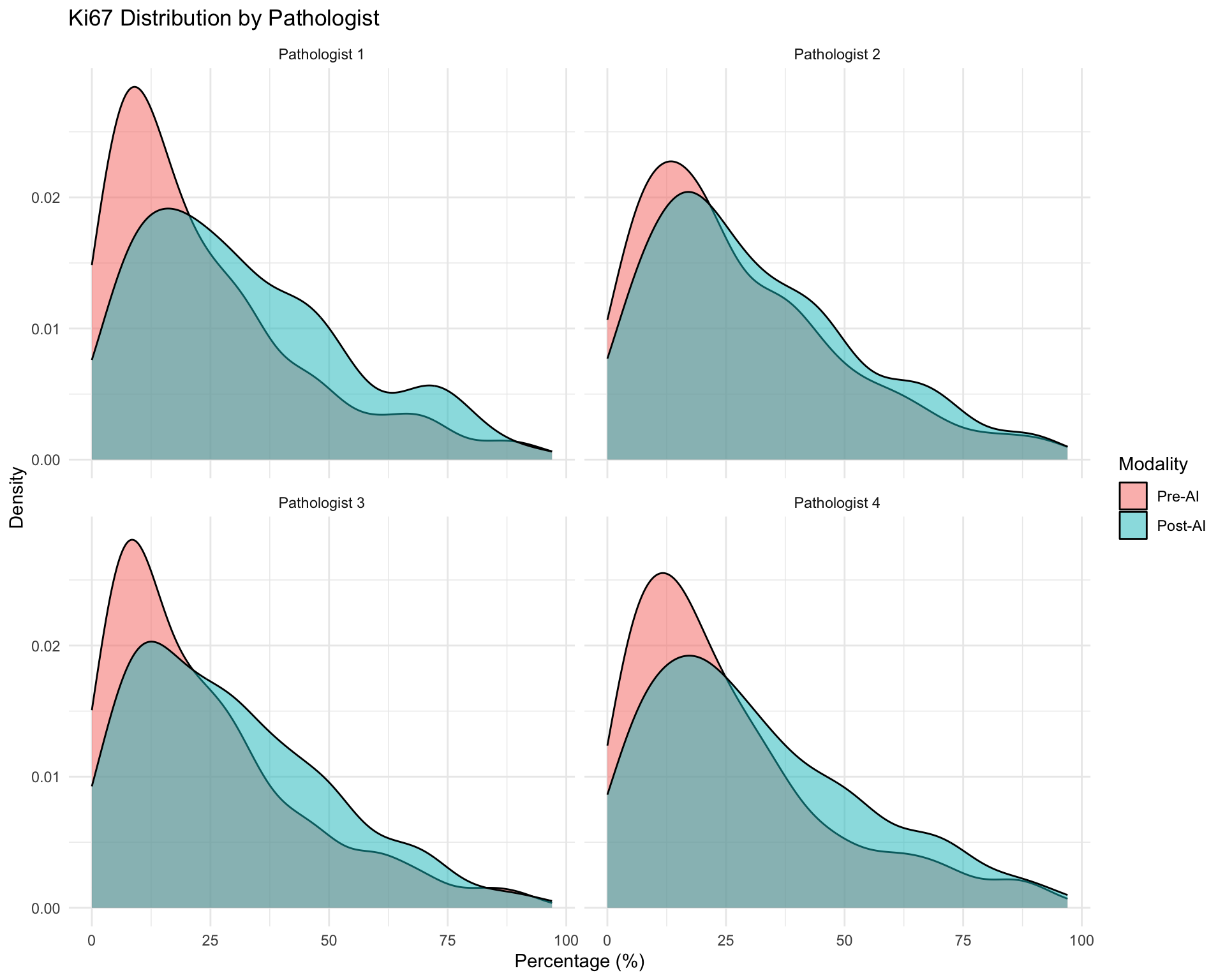
Note for Pathologist: These density plots show the spread of ER, PR, and Ki67 values for each pathologist before and after AI assistance. If the Pre-AI and Post-AI curves overlap closely, the pathologist’s scoring was largely unchanged. If the curves shift, AI influenced their assessments. Pay attention to whether the overall shape (bimodal vs unimodal) changes.
| Characteristic |
ER
|
PR
|
Ki67
|
|||
|---|---|---|---|---|---|---|
| Pre-AI N = 1,183 |
Post-AI N = 1,175 |
Pre-AI N = 1,179 |
Post-AI N = 1,160 |
Pre-AI N = 1,175 |
Post-AI N = 1,162 |
|
| value | ||||||
| Mean (SD) | 72 (37) | 71 (37) | 31 (37) | 31 (35) | 25 (21) | 31 (22) |
| Median (Q1, Q3) | 90 (70, 95) | 90 (60, 95) | 10 (0, 70) | 10 (0, 66) | 20 (10, 35) | 27 (14, 45) |
| Min, Max | 0, 100 | 0, 100 | 0, 100 | 0, 100 | 0, 96 | 0, 97 |
Note for Pathologist: The summary table shows means, medians, and ranges for each continuous marker. Compare the Pre-AI and Post-AI columns: if means shift substantially, AI is systematically pushing values in one direction. The interquartile range (Q1-Q3) tells you where the “middle 50%” of values fall.
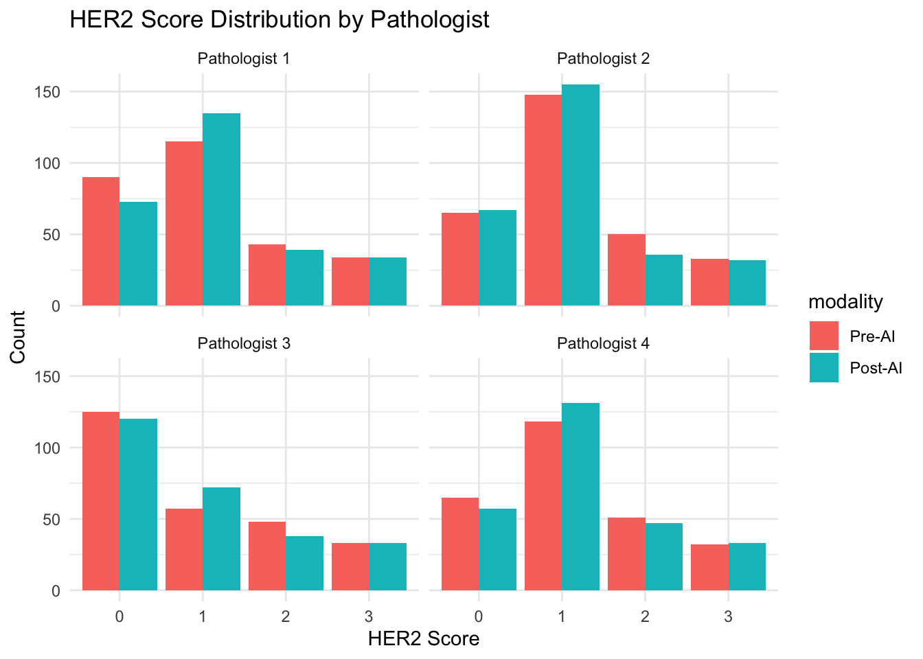
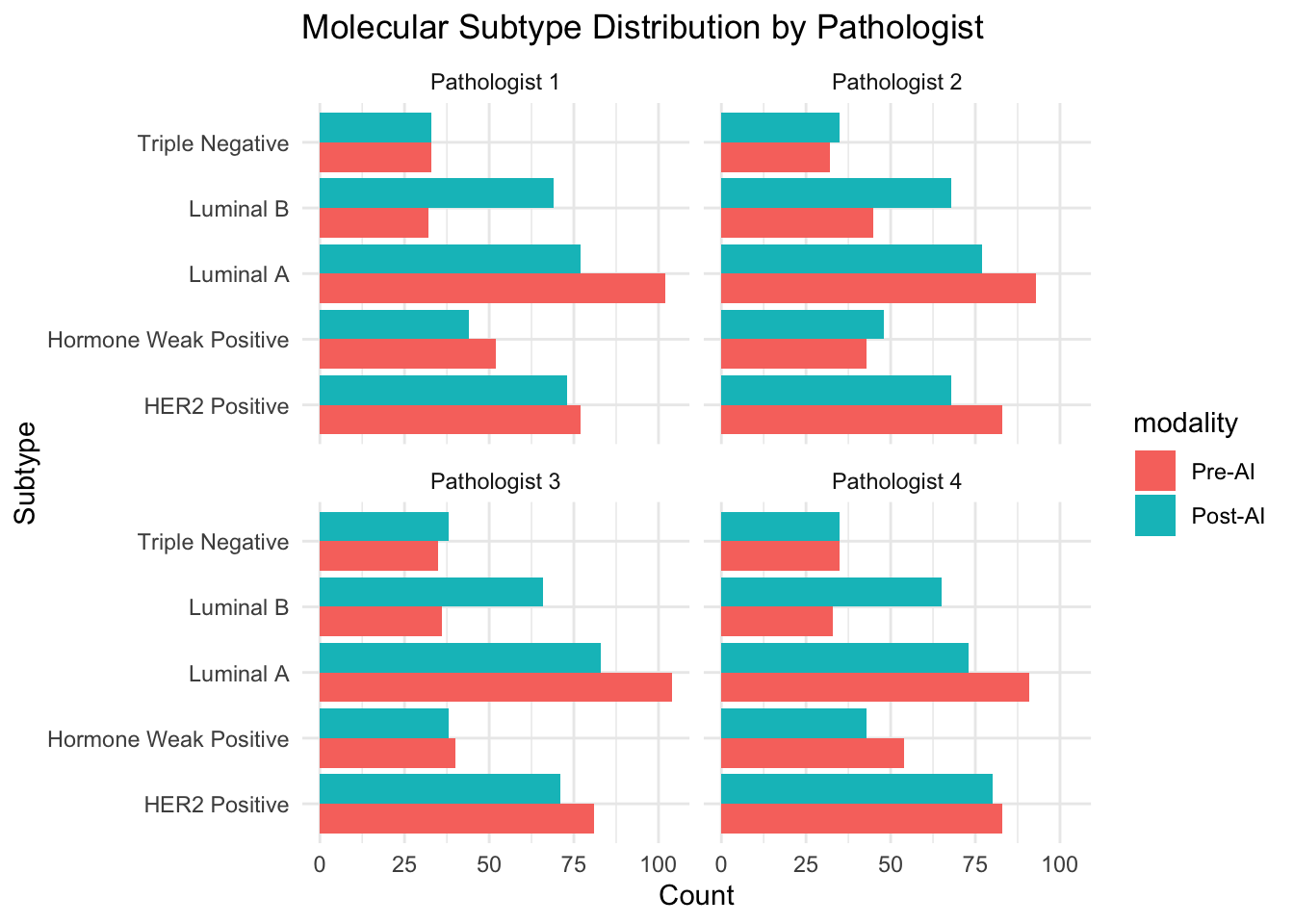
Note for Pathologist: The bar charts for HER2 and molecular subtypes show the number of cases in each category. Side-by-side Pre-AI and Post-AI bars let you see if AI shifted the distribution – for example, if more cases were scored HER2 2+ after AI, that means more FISH tests would be triggered.
We visualize how classifications changed after AI assistance using alluvial plots (approximated here with crosstabs for clarity) or simple transition matrices.
| ER Category Transitions (Pre -> Post) | ||
| Pre-AI | Post-AI | Count |
|---|---|---|
| Negative | Negative | 185 |
| Negative | Low | 9 |
| Low | Low | 15 |
| Low | Positive | 8 |
| Positive | Low | 4 |
| Positive | Positive | 954 |
| PR Category Transitions (Pre -> Post) | ||
| Pre-AI | Post-AI | Count |
|---|---|---|
| Negative | Negative | 420 |
| Negative | Low | 30 |
| Negative | Positive | 3 |
| Low | Negative | 6 |
| Low | Low | 92 |
| Low | Positive | 19 |
| Positive | Low | 13 |
| Positive | Positive | 576 |
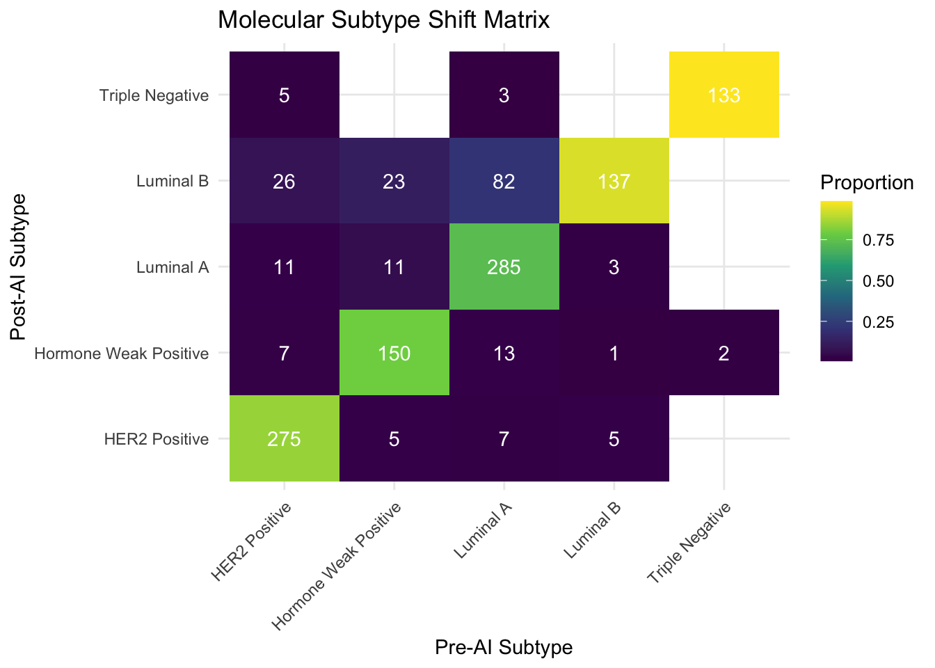
Note for Pathologist: The heatmap above shows how molecular subtypes shifted after AI. Diagonal cells (e.g., Luminal A to Luminal A) represent cases that stayed the same. Off-diagonal cells show reclassifications. Brighter colors indicate more frequent transitions. The most clinically important transitions are between Luminal A and Luminal B (affecting chemotherapy decisions) and any shift to or from Triple Negative.